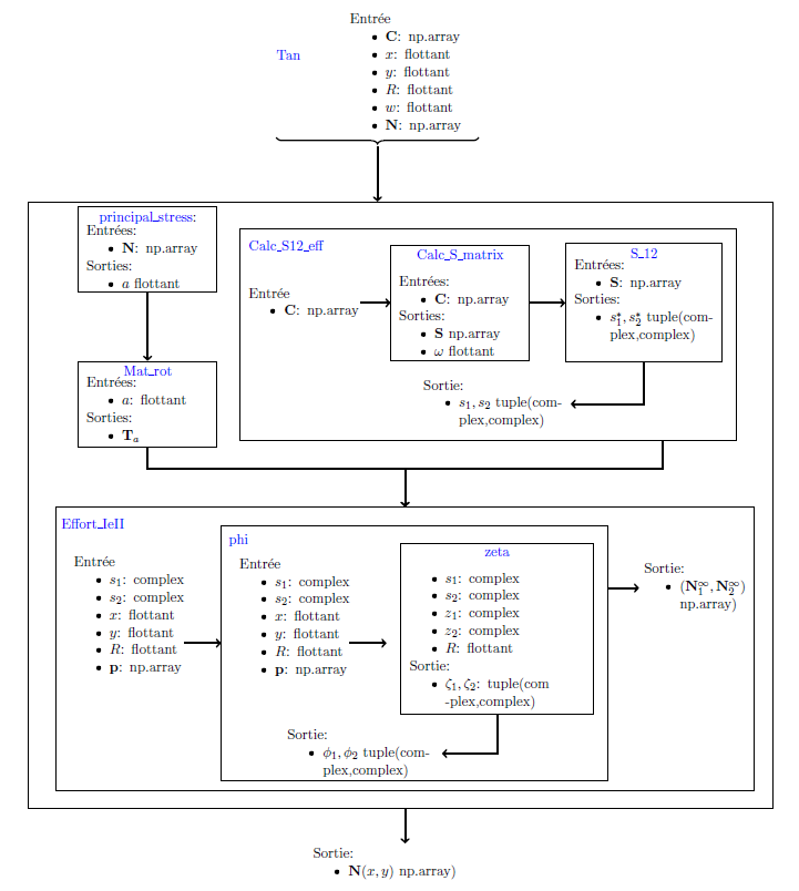
Tan Model Equations

Principal stress coordinate system

The coordinate system (x,y) is rotated to the principal stress frame (1,2).

The rotation angle is:

\[ \alpha = \begin{cases} \frac{1}{2}\arctan\left(\frac{N_{xy}}{N_{xx}-N_{yy}}\right) & if N_{xx}\neq N_{yy} \\ \frac{\pi}{4} & \text{otherwise} \end{cases} \]

Load transformation

The load vector is transformed using a rotation matrix:

\[ p = T_\alpha N \]

where \(T_\alpha\) is the rotation matrix.

Stress field computation

In this coordinate system, the membrane stress solution for an infinite anisotropic plate with a hole in its thickness is determined using a complex method. For each load component, p1 and p2, there is a membrane stress field denoted respectively as \(N_1(x, y)\) and \(N_2(x, y)\). These are expressed as the combination of a uniform membrane stress and a stress resulting from the hole. For any point with coordinates (x, y) in the initial coordinate system, the solution fields are expressed as follows.

The field driven by the load component \(p_1\) is

\[ N_1(x,y) = \begin{pmatrix} p_1 + 2\,\mathrm{Re}\!\left(s_1^2\,\phi_1^{(1)} + s_2^2\,\phi_2^{(1)}\right) \\[4pt] 2\,\mathrm{Re}\!\left(\phi_1^{(1)} + \phi_2^{(1)}\right) \\[4pt] -2\,\mathrm{Re}\!\left(s_1\,\phi_1^{(1)} + s_2\,\phi_2^{(1)}\right) \end{pmatrix}, \]

and the field driven by the load component \(p_2\) is

\[ N_2(x,y) = \begin{pmatrix} 2\,\mathrm{Re}\!\left(s_1^2\,\phi_1^{(2)} + s_2^2\,\phi_2^{(2)}\right) \\[4pt] p_2 + 2\,\mathrm{Re}\!\left(\phi_1^{(2)} + \phi_2^{(2)}\right) \\[4pt] -2\,\mathrm{Re}\!\left(s_1\,\phi_1^{(2)} + s_2\,\phi_2^{(2)}\right) \end{pmatrix}, \]

where each vector collects the \((N_{xx}, N_{yy}, N_{xy})\) components and \(\mathrm{Re}(\cdot)\) is the real part. The complex potentials \(\phi_j^{(k)}\) (root \(j \in \{1,2\}\), load component \(k \in \{1,2\}\)) are

\[ \begin{aligned} \phi_1^{(1)} &= \frac{-i\,p_1\,\bigl(1 - \zeta_1\bigr)}{2\,(s_1 - s_2)\,(1 + i\,s_1)}, & \phi_2^{(1)} &= \frac{i\,p_1\,\bigl(1 - \zeta_2\bigr)}{2\,(s_1 - s_2)\,(1 + i\,s_2)}, \\[6pt] \phi_1^{(2)} &= \frac{p_2\,s_2\,\bigl(1 - \zeta_1\bigr)}{2\,(s_1 - s_2)\,(1 + i\,s_1)}, & \phi_2^{(2)} &= \frac{-p_2\,s_1\,\bigl(1 - \zeta_2\bigr)}{2\,(s_1 - s_2)\,(1 + i\,s_2)}, \end{aligned} \]

with the auxiliary mapping functions

\[ \zeta_j(x,y) = \frac{z_j}{\sqrt{z_j^2 - R^2\,(1 + s_j^2)}}, \qquad z_j(x,y) = x + s_j\,y, \quad j \in \{1,2\}, \]

where the branch of the square root is chosen so that \(\mathrm{Re}(\zeta_j) \geq 0\). The characteristic roots \(s_1\) and \(s_2\) are obtained from the effective compliance matrix (see the following section).

Superposition and finite-width correction

The two fields are combined by superposition and rotated back to the coordinate system of the original load to obtain the membrane stress field for an infinite plate:

\[ N_\infty(x,y) = T_\alpha^{-1}\,\bigl(N_1(x,y) + N_2(x,y)\bigr). \]

Because the theoretical formulation assumes an infinite plate, a correction factor \(C\) is applied to account for the finite plate width \(w\):

\[ N(x,y) = C\,N_\infty(x,y), \qquad C = \frac{2 + (1-u)^3}{3 - 3u}, \quad u = \frac{2R}{w}. \]

This factor is a theoretical value for quasi-isotropic materials and is extended to all types of laminates.

Degenerate quasi‑isotropic case

When the laminate approaches in‑plane isotropy, two distinct singularities appear in the formulation. The implementation regularises each one deterministically rather than by perturbing the stiffness matrix, so that the result stays reproducible across platforms and BLAS back‑ends.

Undefined orthotropy frame

The orthotropy axis angle \(\omega\) is normally identified from the extension–shear coupling terms and the \(C_{11}-C_{22}\) asymmetry of the stiffness matrix, essentially as

\[ \omega \sim \arctan\!\left(\frac{\text{coupling}}{\text{asymmetry}}\right). \]

For a quasi‑isotropic laminate both the coupling and the asymmetry vanish, so this ratio becomes an ill‑defined \(0/0\). The orthotropy axes are then genuinely undefined — every rotation leaves the stiffness invariant. When both quantities fall below a relative tolerance (\(10^{-9}\,\lVert C\rVert\)), the frame is fixed to the arbitrary but exact choice \(\omega = 0\), i.e. the current coordinate frame is kept.

Coincident characteristic roots

The complex potentials \(\phi_1\) and \(\phi_2\) divide by \(s_1 - s_2\), which vanishes at the isotropic double root \(s_1 = s_2 = i\). The stress field has a finite (removable) limit there, but the direct evaluation loses all precision once \(\lvert s_1 - s_2\rvert\) drops below \(\sim 10^{-6}\), and yields NaN at exactly zero.

To keep the computation well conditioned, the separation of the roots is floored to a minimum value \(\delta_{\min} = 10^{-4}\). The two roots are pushed symmetrically apart about their midpoint, along the physical direction of the separation:

\[ s_{1,2} \leftarrow \frac{s_1 + s_2}{2} \pm \frac{\delta_{\min}}{2}\, \frac{s_1 - s_2}{\lvert s_1 - s_2\rvert}, \quad \text{when } \lvert s_1 - s_2\rvert < \delta_{\min}. \]

For an exactly double root the separation direction is undefined and the imaginary axis is chosen (both roots sit near \(+i\)). Because the stress field is continuous in \((s_1, s_2)\), the bias introduced by this flooring is of the order of \(\delta_{\min}\) and negligible for engineering purposes.

Computational steps